The Introduction ends with a question: which choices change the answer, and by how much? This stage answers it with one comparison. Every choice we tested is run against the main map (D8 connectivity at 25 m or 100 m, LIST 2021 land-use pressure averaged over each named system, slope multiplier 0.5 to 1) and scored with one measure, the rank correlation over the mapped karst cells: 1 means the same ordering of cells, lower means a bigger change.
Choices are grouped under the three tests of the project:
| Group | Choices |
|---|---|
| Scale | Routing on a 2 m DEM (Mole Creek only); the 100 m grid against 25 m (Mole Creek only) |
| Data | DEA 2020 land cover instead of LIST land use |
| Method | The same four ingredients added instead of multiplied; six inputs added as a weighted sum; a slope ceiling of 10 degrees; COP’s Scenario 2 slope direction; exposure removed from susceptibility (susceptibility = intensity only) |
Details of each test are in Stages 8, 9, 13 and 14; this stage only brings the numbers together on one measure.
from pathlib import Path
import os, sys
import numpy as np
import pandas as pd
import geopandas as gpd
import rasterio
from rasterio.mask import mask
from rasterio.warp import reproject, Resampling
from scipy.stats import spearmanr
import matplotlib.pyplot as plt

sys.path.insert(0, str(Path("..") / "src"))
from karst import (add_karst_susceptibility, add_connectivity, add_connectivity_d8, rasterize_max,
                   in_mole_creek_focus, mole_creek_focus_mask, aggregate_pressure_by_system, susceptibility_score)
from hydro import slope_degrees, slope_risk_multiplier, score_watercourses
from landuse import fetch_landuse_pressure
from landuse_list import MATRIX, load_list_landuse, pressure_raster
from structures import weighted_sum, build_inputs, W_EQUAL

data = Path(os.environ.get("AT3_DATA_DIR", "data"))
inpath = data / "Input_data"
outpath = data / "Output_data"
LIST_2021 = inpath / "LIST_LAND_USE_2021_STATEWIDE" / "list_land_use_2021_statewide.shp"
LIST_TOP = float(max(MATRIX.values()))
COP_EDGES = [float(np.degrees(np.arctan(p / 100))) for p in (8, 31, 76)]

def cop_scenario2(slope_deg):
    """COP Scenario 2: flatter = higher, four classes at 8%, 31%, 76%, scaled 1 down to 0.5."""
    cls = np.digitize(np.nan_to_num(slope_deg), COP_EDGES)
    return np.where(np.isnan(slope_deg), 1.0, np.array([1.0, 5 / 6, 4 / 6, 0.5])[cls])

def variants(S, C, P_main, m, extras):
    """Risk rasters for every choice. S, C, P in 0-1, m the slope multiplier; `extras` carries the alternatives."""
    slope_in = (m - 0.5) / 0.5
    gate = S > 0
    out = {
        "main": S * C * P_main * m,
        "Data: DEA land cover": S * C * extras["P_dea"] * m,
        "Method: four ingredients added": np.where(gate, (S + C + P_main + slope_in) / 4, 0.0),
        "Method: six ingredients added": weighted_sum(extras["X"], W_EQUAL) * P_main,
        "Method: exposure removed": extras["S_noexp"] * C * P_main * m,
        "Method: slope, 10 degree ceiling": S * C * P_main * slope_risk_multiplier(extras["slope_deg"], ref_deg=10),
        "Method: slope, flatter = higher": S * C * P_main * cop_scenario2(extras["slope_deg"]),
    }
    if "C_2m" in extras:
        out["Scale: 2 m DEM"] = S * extras["C_2m"] * P_main * m
    return out

def rank_corr(risks, karst_mask):
    base = risks["main"]
    rows = {}
    for name, r in risks.items():
        if name == "main":
            continue
        ok = karst_mask & np.isfinite(base) & np.isfinite(r)
        rows[name] = spearmanr(base[ok], r[ok])[0]
    return rows
16.1 Mole Creek (25 m)
with rasterio.open(outpath / "karst_intensity_mc_EPSG7855.tif") as src:
    intensity = src.read(1).astype(float)
with rasterio.open(outpath / "karst_exposure_mc_EPSG7855.tif") as src:
    exposure = src.read(1).astype(float)
with rasterio.open(outpath / "connectivity_mc_EPSG7855.tif") as src:
    conn_mc = src.read(1).astype(float)
with rasterio.open(outpath / "landuse_pressure_mc_2020_EPSG7855.tif") as src:
    p2020 = src.read(1).astype(float); p_nodata = src.nodata   # DEA 2020 land cover, the alternative
with rasterio.open(outpath / "dem_mc_EPSG7855.tif") as src:
    dem = src.read(1); dem_nodata = src.nodata; transform = src.transform; shape = dem.shape; cell = abs(src.transform.a); bounds = src.bounds

karst_mc = gpd.read_file(outpath / "karst_mc_connectivity_EPSG7855.gpkg")
karst_mc = karst_mc[karst_mc.geom_type.isin(["Polygon", "MultiPolygon"])].copy()
focus = mole_creek_focus_mask(karst_mc, shape, transform)
focus_valid = (dem != dem_nodata) & focus

slope_deg = slope_degrees(dem, dem_nodata, cell)
m_main = slope_risk_multiplier(slope_deg)
S = susceptibility_score(intensity, exposure)   # main susceptibility: karst intensity x exposure
S_noexp = intensity / 4.0                       # the same without exposure, for the sensitivity row
C = conn_mc / 3.0
eff2020 = aggregate_pressure_by_system(karst_mc, p2020, transform, p_nodata)
P_dea = np.where(p2020 != p_nodata, eff2020 / 3.0, np.nan)

lu = load_list_landuse(LIST_2021, "EPSG:7855", bounds_target=tuple(bounds))
p_list = pressure_raster(lu, MATRIX, shape, transform).astype(float)
eff_list = aggregate_pressure_by_system(karst_mc, p_list, transform, -1)
P_main = np.where(eff_list >= 0, eff_list / LIST_TOP, np.nan)
valid = focus_valid & (p_list >= 0)
karst_cells = valid & (intensity > 0)

# six-input weighted sum inputs
wc = gpd.read_file(outpath / "watercourses_tas_EPSG7855.gpkg")
wc = score_watercourses(wc[wc["HYDLNTY1"] == "Watercourse"] if "HYDLNTY1" in wc.columns else wc)
mc_b = gpd.read_file(outpath / "mole_creek_bounding_box_EPSG7855.gpkg").total_bounds
wc_mc = wc.cx[mc_b[0]:mc_b[2], mc_b[1]:mc_b[3]]
karst_all = gpd.read_file(inpath / "KarstAtlas/Karst_Ver_3_1/Karst_Atlas_v3_1.shp")
rain_range = (karst_all.loc[karst_all["KCATEGORY"].isin(list("ABCD")), "KAVRAIN"].min(), karst_all.loc[karst_all["KCATEGORY"].isin(list("ABCD")), "KAVRAIN"].max())
X = build_inputs(karst_mc, shape, transform, wc_mc, slope_deg, rain_range)

# routing on the 2 m DEM
k2 = karst_mc.copy()
add_connectivity_d8(k2, outpath / "karst_upstream_connectivity_counts_core_mc_2m_EPSG7855_jenks5.csv", scheme="decades")
C_2m = rasterize_max(k2, "connectivity", shape, transform, dtype="float32").astype(float) / 3.0

extras = {"S_noexp": S_noexp, "P_dea": P_dea, "X": X, "slope_deg": slope_deg, "P_raw": np.where(p_list >= 0, p_list / LIST_TOP, np.nan), "C_2m": C_2m}
risks = {k: np.where(valid, v, np.nan) for k, v in variants(S, C, P_main, m_main, extras).items()}

# the 100 m statewide run, resampled to this grid (as in Stage 8)
with rasterio.open(outpath / "risk_tas_2020_100m_EPSG7855.tif") as src:
    coarse = np.full(shape, src.nodata, dtype="float32")
    reproject(rasterio.band(src, 1), coarse, src_transform=src.transform, src_crs=src.crs, dst_transform=transform,
              dst_crs=src.crs, resampling=Resampling.nearest, src_nodata=src.nodata, dst_nodata=src.nodata)
    nd = src.nodata
risks["Scale: 100 m DEM"] = np.where(valid & (coarse != nd), coarse, np.nan)

corr_mc = rank_corr(risks, karst_cells)
print(f"Mole Creek: {int((karst_cells & np.isfinite(risks['main'])).sum()):,} karst cells")
print(pd.Series(corr_mc).round(3).sort_values().to_string())
Mole Creek: 412,523 karst cells
Method: six ingredients added 0.549
Method: slope, flatter = higher 0.825
Scale: 100 m DEM 0.894
Method: exposure removed 0.907
Data: DEA land cover 0.979
Method: four ingredients added 0.979
Method: slope, 10 degree ceiling 0.992
Scale: 2 m DEM 0.994
16.2 Statewide (100 m)
tasmania = gpd.read_file(outpath / "tasmania_bounding_box_EPSG7855.gpkg")
tmpl = outpath / "dem_tas_100m_EPSG7855.tif"
with rasterio.open(tmpl) as src:
    tdem = src.read(1).astype(float); tnodata = src.nodata; ttransform = src.transform; tshape = tdem.shape
    land, _ = mask(src, tasmania.geometry, crop=False, nodata=tnodata)
tvalid_land = land[0] != tnodata

karst_tas = gpd.read_file(outpath / "karst_tas_EPSG7855.gpkg")
add_karst_susceptibility(karst_tas); add_connectivity(karst_tas)
add_connectivity_d8(karst_tas, outpath / "karst_upstream_connectivity_counts_tas_100m_EPSG7855.csv", scheme="decades")
t_int = rasterize_max(karst_tas, "karst_intensity", tshape, ttransform).astype(float)
t_conn = rasterize_max(karst_tas, "connectivity", tshape, ttransform, dtype="float32").astype(float)
t_expo = rasterize_max(karst_tas, "exposure_code", tshape, ttransform).astype(float)
tS, tC = susceptibility_score(t_int, t_expo), t_conn / 3.0
tS_noexp = t_int / 4.0

bbox = tasmania.to_crs("EPSG:4326").total_bounds.tolist()
cache = inpath / "DEA_Land_Cover_Cache"
tp2020 = fetch_landuse_pressure(bbox, 2020, tmpl, target_crs="EPSG:7855", cache_dir=cache).astype(float)
teff2020 = aggregate_pressure_by_system(karst_tas, tp2020, ttransform, 255)
tP_dea = np.where(tp2020 != 255, teff2020 / 3.0, np.nan)
lu_t = load_list_landuse(LIST_2021, "EPSG:7855")
tp_list = pressure_raster(lu_t, MATRIX, tshape, ttransform).astype(float)
teff_list = aggregate_pressure_by_system(karst_tas, tp_list, ttransform, -1)
tP_main = np.where(teff_list >= 0, teff_list / LIST_TOP, np.nan)
tvalid = tvalid_land & (tp_list >= 0)

tslope = slope_degrees(tdem, tnodata, abs(ttransform.a))
tm = slope_risk_multiplier(tslope)
rain_range_t = (karst_tas.loc[karst_tas["karst_intensity"] > 0, "KAVRAIN"].min(), karst_tas.loc[karst_tas["karst_intensity"] > 0, "KAVRAIN"].max())
TX = build_inputs(karst_tas, tshape, ttransform, wc, tslope, rain_range_t)

textras = {"S_noexp": tS_noexp, "P_dea": tP_dea, "X": TX, "slope_deg": tslope, "P_raw": np.where(tp_list >= 0, tp_list / LIST_TOP, np.nan)}
trisks = {k: np.where(tvalid, v, np.nan) for k, v in variants(tS, tC, tP_main, tm, textras).items()}
corr_tas = rank_corr(trisks, tvalid & (t_int > 0))
print(f"Tasmania: {int((tvalid & (t_int > 0) & np.isfinite(trisks['main'])).sum()):,} karst cells")
print(pd.Series(corr_tas).round(3).sort_values().to_string())
Tasmania: 410,000 karst cells
Method: four ingredients added 0.704
Method: six ingredients added 0.821
Data: DEA land cover 0.843
Method: slope, flatter = higher 0.955
Method: exposure removed 0.963
Method: slope, 10 degree ceiling 0.987
16.3 The chart
table = pd.DataFrame({"Mole Creek (25 m)": pd.Series(corr_mc), "Tasmania (100 m)": pd.Series(corr_tas)})
table["group"] = [n.split(":")[0] for n in table.index]
table["choice"] = [n.split(": ", 1)[1] for n in table.index]
table["sort"] = table[["Mole Creek (25 m)", "Tasmania (100 m)"]].min(axis=1)
# grouped Scale, Data, Method; within a group the biggest change first, except Scale reads 2 m then 100 m
ORDER = ["Scale: 2 m DEM", "Scale: 100 m DEM", "Data: DEA land cover", "Method: four ingredients added",
         "Method: six ingredients added", "Method: slope, flatter = higher", "Method: slope, 10 degree ceiling",
         "Method: exposure removed"]
table = table.reindex([o for o in ORDER if o in table.index])
table["choice"] = [c[0].upper() + c[1:] for c in table["choice"]]
table.drop(columns="sort").round(3).to_csv(outpath / "stage16_choices_rank_correlation.csv")
print(table.drop(columns=["sort"]).round(3).to_string())

GROUP_COLOURS = {"Scale": "#2a6fb0", "Data": "#b9822f", "Method": "#b5434e"}
fig, ax = plt.subplots(figsize=(10.5, 6.4))
ypos = np.arange(len(table))
for y, (_, row) in zip(ypos, table.iterrows()):
    colour = GROUP_COLOURS[row["group"]]
    a, b = row["Mole Creek (25 m)"], row["Tasmania (100 m)"]
    if np.isfinite(a) and np.isfinite(b):
        ax.plot([a, b], [y, y], color=colour, lw=2, alpha=0.5, zorder=1)
    if np.isfinite(a):
        ax.scatter(a, y, s=70, color=colour, marker="o", zorder=3)
    if np.isfinite(b):
        ax.scatter(b, y, s=70, color=colour, marker="s", zorder=3)
ax.set_yticks(ypos)
ax.set_yticklabels([f"{r['choice']}" for _, r in table.iterrows()], fontsize=10)
for tick, (_, row) in zip(ax.get_yticklabels(), table.iterrows()):
    tick.set_color(GROUP_COLOURS[row["group"]])
low = float(np.floor(min(0.0, table[['Mole Creek (25 m)', 'Tasmania (100 m)']].min().min()) * 10) / 10)
ax.set_xlim(low - 0.02, 1.02)
ax.invert_yaxis()
ax.axvline(1.0, color="#999999", lw=1, ls="--")
if low < 0:
    ax.axvline(0.0, color="#bbbbbb", lw=1)
ax.set_xlabel("Rank correlation with the main map over the mapped karst (1 = same ordering; lower = bigger change)", fontsize=10)
ax.grid(axis="x", color="#dddddd", lw=0.6)
ax.set_axisbelow(True)
from matplotlib.lines import Line2D
legend = [Line2D([0], [0], marker="o", color="w", markerfacecolor="#444444", markersize=9, label="Mole Creek (25 m)"),
          Line2D([0], [0], marker="s", color="w", markerfacecolor="#444444", markersize=9, label="Tasmania (100 m)")]
legend += [Line2D([0], [0], color=c, lw=6, label=g) for g, c in GROUP_COLOURS.items()]
ax.legend(handles=legend, loc="upper left", fontsize=9, framealpha=0.95, ncol=2)
ax.set_title("How far each choice moves the map", fontsize=13, loc="left")
for side in ("top", "right"):
    ax.spines[side].set_visible(False)
plt.tight_layout()
fig.savefig(Path("..") / "figures" / "choices_that_matter.png", dpi=200, bbox_inches="tight")
plt.show()
Mole Creek (25 m) Tasmania (100 m) group choice
Scale: 2 m DEM 0.994 NaN Scale 2 m DEM
Scale: 100 m DEM 0.894 NaN Scale 100 m DEM
Data: DEA land cover 0.979 0.843 Data DEA land cover
Method: four ingredients added 0.979 0.704 Method Four ingredients added
Method: six ingredients added 0.549 0.821 Method Six ingredients added
Method: slope, flatter = higher 0.825 0.955 Method Slope, flatter = higher
Method: slope, 10 degree ceiling 0.992 0.987 Method Slope, 10 degree ceiling
Method: exposure removed 0.907 0.963 Method Exposure removed
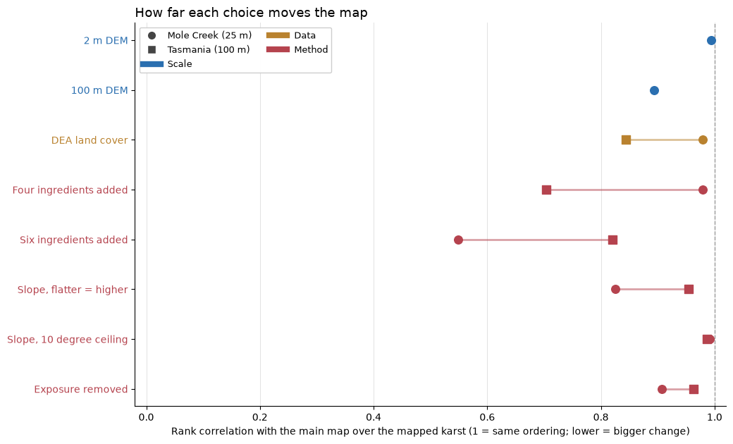
Result: most choices leave the ordering of the karst nearly unchanged, and a few change it a lot.
Little change (rank correlation 0.98 or above): routing on a 2 m DEM (0.99 at Mole Creek), the slope ceiling (0.99 at both), and, at Mole Creek only, DEA land cover in place of LIST (0.98) and adding the same four ingredients instead of multiplying (0.98).
Moderate (0.70 to 0.96): the 100 m grid against 25 m at Mole Creek (0.89), removing exposure (0.91 at Mole Creek, 0.96 statewide), COP’s slope direction (0.83 at Mole Creek, 0.96 statewide) and, statewide, DEA land cover (0.84), the six-input weighted sum (0.82) and adding the same four ingredients (0.70).
Large (below 0.6): the six-input weighted sum at Mole Creek (0.55).
The land-cover year is not tested here: it is a change to track on the final map (Stage 9 shows the pattern stays stable year to year while the level moves). The method choices matter most, meaning which ingredients are added or multiplied, and the slope rule. Adding the same four ingredients keeps the Mole Creek ordering (0.98), while adding six different inputs does not (0.55), so the extra inputs change the map there. Exposure changes the map about as much as the 100 m grid does, and it is part of the main model because it improves the springs check (Stage 10). Mole Creek moves more than the state under several choices because it is a small, closely mapped area where one or two systems set the ordering.