How do we get there?
Karst Intrinsic Vulnerability Index (KIVI) method
After consideration of karst vulnerability index methods from the literature and investigation of available datasets, we decided on a multiplicative index using 3 parameters based on EPIK. EPIK uses the parameters:
Epikarst - the upper 3-30m layer of a karst environment where part of the water is stored and released slowly while the rest flows into the endokarst below
Protective cover - the sediment overlying the karst rock
Infiltration conditions - the type of recharge to the karst aquifer
Karst network development - the subsurface cave system development and connectivity (Doerfliger et al, 1999)
We used 3 parameters for the Karst Intrinsic Vulnerability Index (KIVI) :
1. Karst intensity - Karst Atlas attribute Kcategory which we scored 4-1 for A-D, which has aspects of EPIK’s epikarst and karst network development.
Table 1:Karst categories from Tasmanian Karst Atlas v3.1
| Characters | Karst Categories | Karst intensity |
|---|---|---|
| A | intensely karstified or probably intensively karstified. | 4 |
| B | substantially karstified or probably substantially karstified. | 3 |
| C | partially karstified or potentially partly karstified. | 2 |
| D | possibly partially karstified. | 1 |
2. Karst exposure - Karst Atlas Kexposed, Kcovered or Kinterstr scored 3, 2 and 1 which directly relates to EPIK’s protective cover parameter. Exposed has no or only thin layers of soil above the karst rock, covered has substantial but unlithified deposits above it and interstr(atal) has lithified rock above it (Sharples, 2003).
3. Connectivity - relates to EPIK’s infiltration conditions. EPIK’s infiltration scores include a coefficient based on slope and vegetative cover however because we wanted to be able to add slope and vegetation as separate parameters we didn’t include them here. Connectivity was calculated by counting the upstream cells directly connected to each karst polygon by following the Whitebox D8 point upstream, and changing that to a target cell ratio per polygon. These were classed into four powers-of-ten ranges and scored 0 to 3 after rescaling.
The final KIVI score came from normalising each parameter to give a score between 0 and 1 and multiplying the 3 together.
Source datasets
Australian Bureau of Statistics STE_2021_AUST_SHP_GDA2020
DEA Level 3 Land Cover
Geology at 1:25,000 (Mineral Resources Tasmania)
Lands Tasmania 2m DEM downloaded from the ELVIS platform
LIST CFEV Groundwater Statewide
LIST CFEV Karst Statewide
LIST DEM 25m
LIST Hydline
LIST Land Use
Tasmanian Digital Karst Atlas Version 3.1 GIS data set
Study areas: 1. Mole Creek 2. Tasmania including offshore islands
CRS: GDA2020 / MGA Zone 55 (EPSG:7855)
Python libraries used
| Python Libraries | What they were used for |
|---|---|
| GeoPandas and Shapely | Read, reproject, filter and analyse spatial vector data such as Karst Atlas polygons, land-use polygons and watercourses; perform geometry operations such as buffering. |
| Rasterio and rioxarray | Read, write, mosaic, mask, rasterize and align raster data; manage raster grids, coordinate systems, NoData values and resampling. |
| NumPy | Store raster data as arrays and calculate scores, masks, vulnerability and risk cell by cell. |
| Pandas | Manage attribute tables and connectivity count tables; read and write CSVs. |
WhiteboxTools (whitebox) | Prepare the DEM for D8 flow routing and generate flow direction and accumulation products. |
| Numba | Speed up the custom upstream-routing counts used to calculate connectivity. |
| SciPy | Support analyses such as distance calculations and statistical comparisons. |
| pystac-client and odc-stac | Find and load DEA land-cover data from its STAC catalogue. |
| Matplotlib and Contextily | Produce static maps, charts and map backgrounds. |
| Plotly and Folium | Create interactive comparisons and the interactive risk map. |
| Pillow (PIL) and IPython display tools | Handle some image and notebook display tasks. |
GDAL (osgeo.gdal) | Support raster operations in some notebooks. |
We also built our own modules which helped to keep processing consistent across the workflow such as karst.py, hydro.py, landuse.py and d8_routing.py.
Building the model
We built and tuned the method at Mole Creek on a 25 m grid, and then froze it and ran it across all of Tasmania at 100 m. Both use one coordinate system (GDA2020 / MGA55, EPSG:7855). The Mole Creek study area we used was the Karst Atlas polygons with Mole Creek in the name and the Meander - Western Creek polygon, plus a 3 km buffer. This was necessary to include the catchment for the karst polygons for
Raster Preparation (notebooks 00-01)
Bounding boxes for Tasmania and for the Mole Creek area were prepared by reading the source file into a geopandas dataframe, selecting the polygons required and making sure they were in EPSG:7855. The Mole Creek bounding box was used to clip a Mole Creek DEM from the statewide merged and reprojected DEM which was used as the raster grid for the rasterization of the 25m polygons through the workflow. This kept the CRS, grid alignment and explicit NoData handling consistent across the project and between scales.
The parameters, mapped at Mole Creek
1. Susceptibility: how karstified is the rock and how much cover does the karst have? (notebook 02)
Calculating the scores for the susceptibility inputs of karst intensity and exposure is the first step. Each polygon in the Mole Creek karst was given an intensity score and an exposure score and the scores were converted to a raster using the DEM template. You can jump back here to see details of the intensity and exposure classes.
Susceptibility input maps
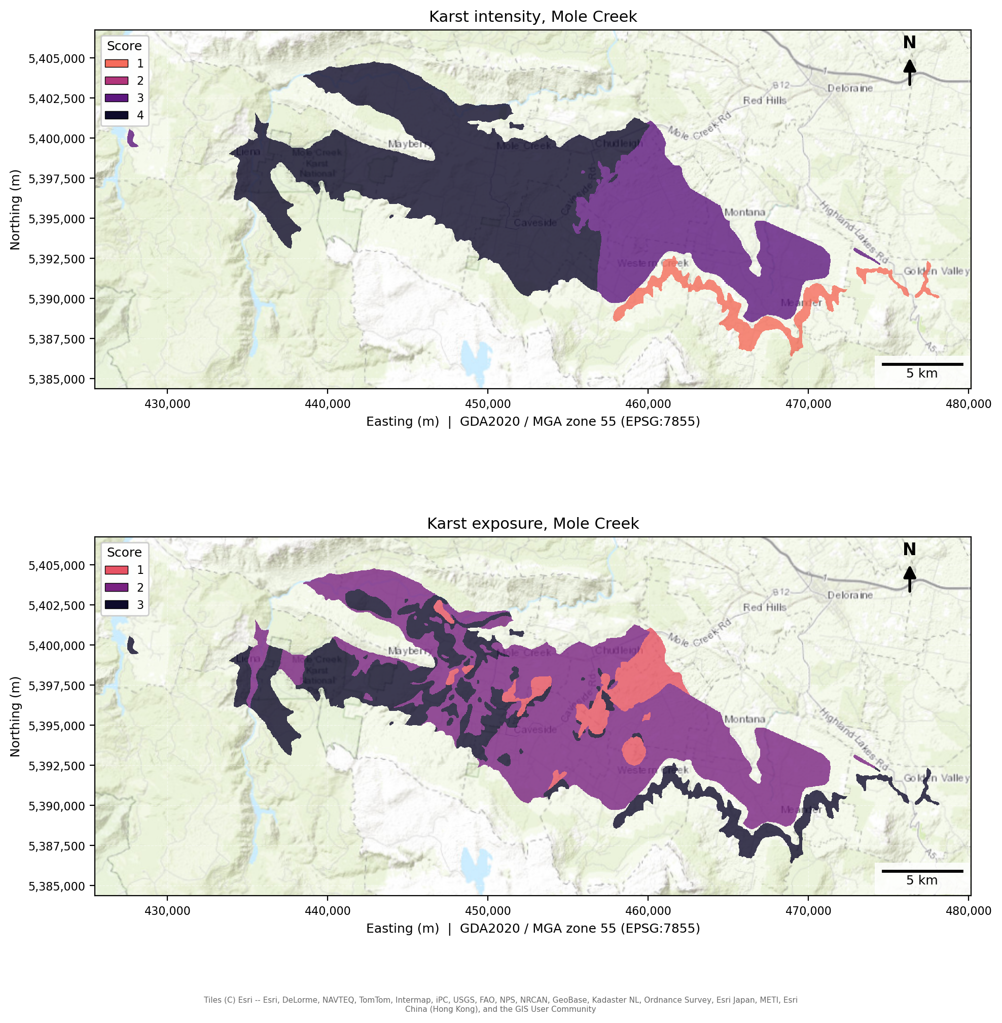
Top, Karst intensity: 1, 2, 3, 4 = possibly partially karstified, partially karstified, substantially karstified, intensely karstified. Bottom, Karst exposure: 1, 2, 3 = interstratal, covered, exposed
2. Connectivity: how much water potentially reaches each polygon? (notebooks 03)
We used the D8 direction map created during the flow accumulation calculation to trace up the hill from each karst polygon and count how many cells could potentially contribute their water to the polygon D8 flow routing (WhiteboxTools) then calculated the ratio of uphill contributing cells per cell of the polygon. All connecting cells on the way to the top of the catchment were counted including the polygon’s own cells, except for interstratal karst as it is not considered to receive the rain falling on it itself.
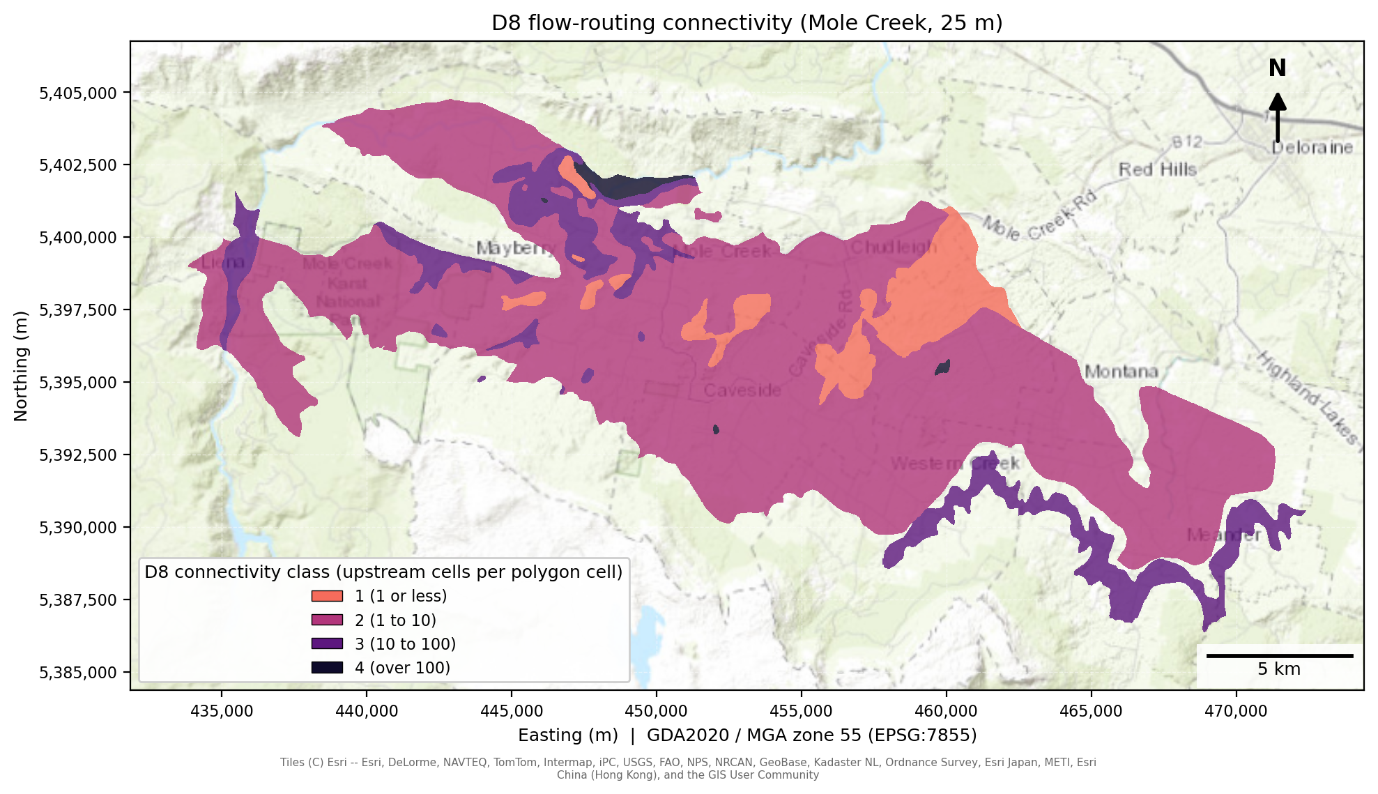
D8 connectivity map for Mole Creek, 25m.
Using the usual fill tool and D8 direction uphill count may not be the best method for an area with highly developed epikarst because it can hide the sinkholes that water flows into. Our logic for using it here was 1. that we needed a method that would work over all types of karst, 2. if the karst is highly interconnected, that water may reach downhill karst anyway just underground and 3. in high intensity/long periods of rainfall much of the rain will flow overground. If we were just focusing on Mole Creek and not wanting to scale the method up to state level there are other flow accumulation methods that retain the sinks and potentially be more accurate from Whitebox and RichDEM. To do this properly would require a more work attempting to map sinkholes more closely through a higher resolution DEM or ground assessment.
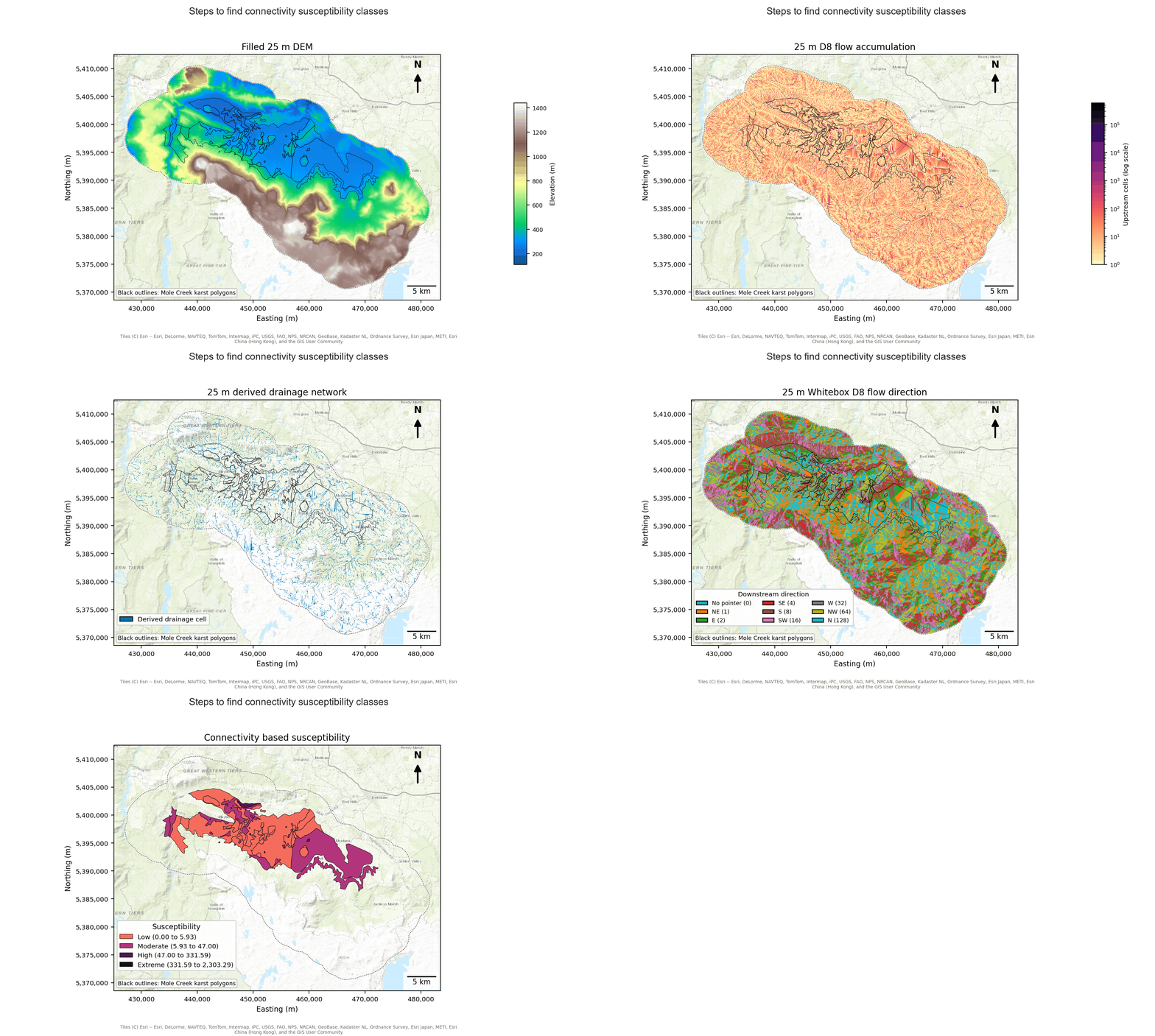
Stages of calculating the hydrological connectivity susceptibility. The gif starts with the DEM.
Karst lower in a large catchment receives more water than karst on a divide. The ratio is classed in powers of ten: class 1 is a ratio of up to 1 contributing cell per polygon cell (little more than the polygon’s own ground drains in), class 2 is 1 to 10, class 3 is 10 to 100, and class 4 is over 100 (hundreds of times its own area, as for a small karst polygon low in a big catchment). The four classes are rescaled to 0 to 3. Each step is ten times the last, which suits a ratio that runs from 0 to over 100,000. The edges are the same at every resolution, so a class means the same ratio at 2 m, 25 m and 100 m, and no single large catchment sets the scale.
Routing depends on the DEM, so connectivity is where resolution enters the project:
| Run | DEM | Area covered | Used for |
|---|---|---|---|
| Fine | 2 m | Mole Creek | Checking the 25 m run |
| Local | 25 m | Mole Creek | The Mole Creek map |
| Statewide | 100 m | All of Tasmania | The Tasmania map |
The 2 m run is too large to repeat for the state, so it is compared with the 25 m run at Mole Creek, and the 100 m run is compared with both on the polygons they share (Stage 13). The Karst Atlas flags give a second connectivity score (the highest of exposure type, proximal catchment and distal catchment), which serves as a check on the routing.
Polygons with no routed score. At 100 m, 132 of the 1,677 karst polygons (about 0.02% of karst area) are too small to hold a single grid cell, so the routing cannot score them. We leave them out: they have no connectivity score and do not appear on the statewide map or in the rankings. Giving them a substitute score, from the Atlas flags or by leaving connectivity out of the product, would score them on a different basis from every other polygon, and would inflate them. At Mole Creek’s 25 m, all 66 polygons are routed. The neighbouring karst inside the 3 km buffer is not routed and is context only.
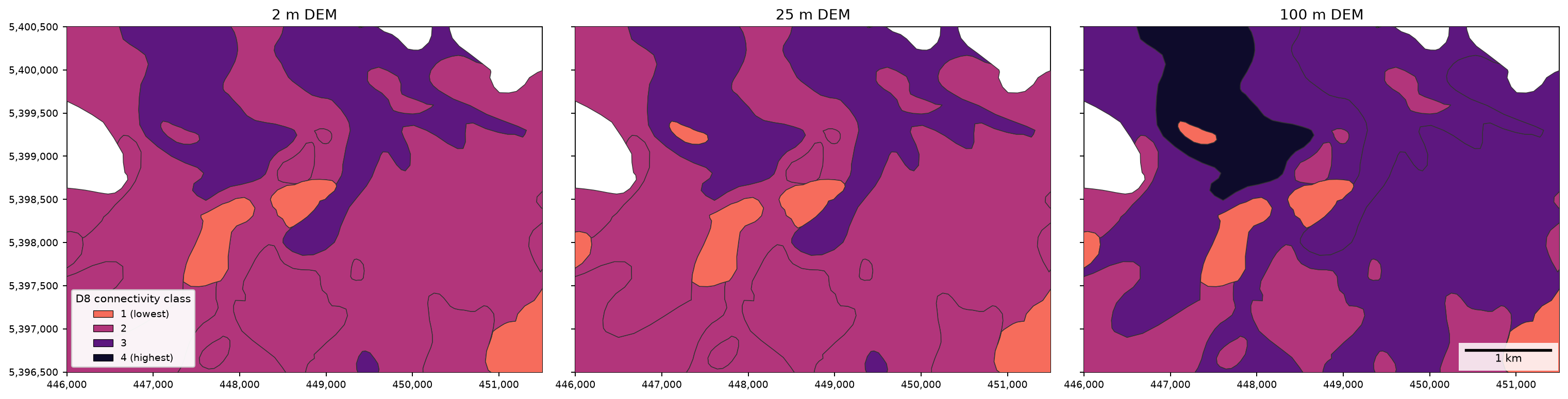
The same ground at three resolutions: the D8 connectivity class of each karst polygon when water is routed on a 2 m, 25 m and 100 m DEM.
3. Calculating KIVI (notebooks 04)
KIVI is calculated at this stage by multiplying susceptibility (intensity x exposure) and D8 connectivity. This gives a continuous index of 12 values which is later reclassified for easier visual comparison.
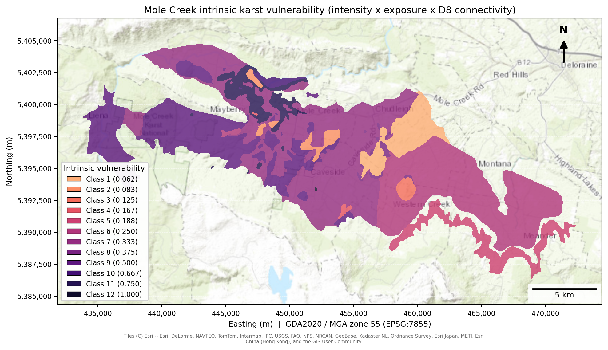
The KIVI for Mole Creek, 25m
4. Pressure: what is on the land?
Karst aquifers are poor at purifying water: at Mole Creek, surface run-off is captured quickly by solutional openings and passes through conduits with little cleaning (Eberhard & Houshold, 2002). What is on the land therefore matters, and there is more than one source of land-use data, so two layers are scored and compared:
| DEA land cover | LIST land use | |
|---|---|---|
| Source | Digital Earth Australia Level 3 land cover (Geoscience Australia, n.d.), annual maps 1988 to 2024, 30 m | LIST Tasmania land-use polygons (2021), 121 classes |
| Classes scored | Six: water, natural vegetation, aquatic vegetation, bare surface, cultivated, artificial | The LIST hierarchy, from conservation land to intensive uses |
| Scale | 0, 1 or 3 | 0 to 10 |
| Sees | Cultivated against natural cover, for any year | Plantation forestry, irrigated pasture, intensive animal production, mining and waste |
| Misses | Cannot separate managed plantation from native forest, and counts lightly grazed pasture as natural | Six snapshots from 2002 to 2021 (fewer than DEA’s annual series), and a heavier Tasmania-only dataset |
The main map uses LIST land use: it is Tasmania’s own source and records what the land is used for as well as what covers it. DEA is kept as a tested alternative.
Land-use pressure at Mole Creek in 2021. Natural land is left clear, and each layer darkens from there up to its own maximum score, so darker means higher pressure within that layer.
Pressure reaches the karst from the catchment. Pressure on the sinkhole cell itself says little, because the water arriving there comes from the whole catchment upslope. Catchment-only polygons also have zero susceptibility, so a per-cell product would ignore their land use entirely, and 26.8% of high-pressure cells at Mole Creek would be missed this way. Each karst cell takes the mean pressure across its named system. We cluster polygons that sit close together, so placeholder names like “Several” do not merge unrelated systems.
Bare ground scores low. It is a natural surface with no pollutant source on it. Fast runoff is already captured by connectivity, so scoring it again here would count it twice.
5. Slope: does runoff concentrate or soak in?
Slope comes from the DEM (25 m at Mole Creek, 100 m statewide). It enters as a multiplier from 0.5 to 1: 0.5 on flat ground, rising in a straight line to 1.0 at 30 degrees or steeper. Steeper ground is scored as more vulnerable, because runoff concentrates and runs towards sinkholes where it falls. The floor of 0.5 keeps flat ground from scoring zero: only “no karst” or “no pressure” gives zero risk. Slope is taken from each run’s own DEM, so the 100 m statewide run sees smoother, gentler slopes than the 25 m local run. The sign and the ceiling are judgements, tested as part of the method test below.
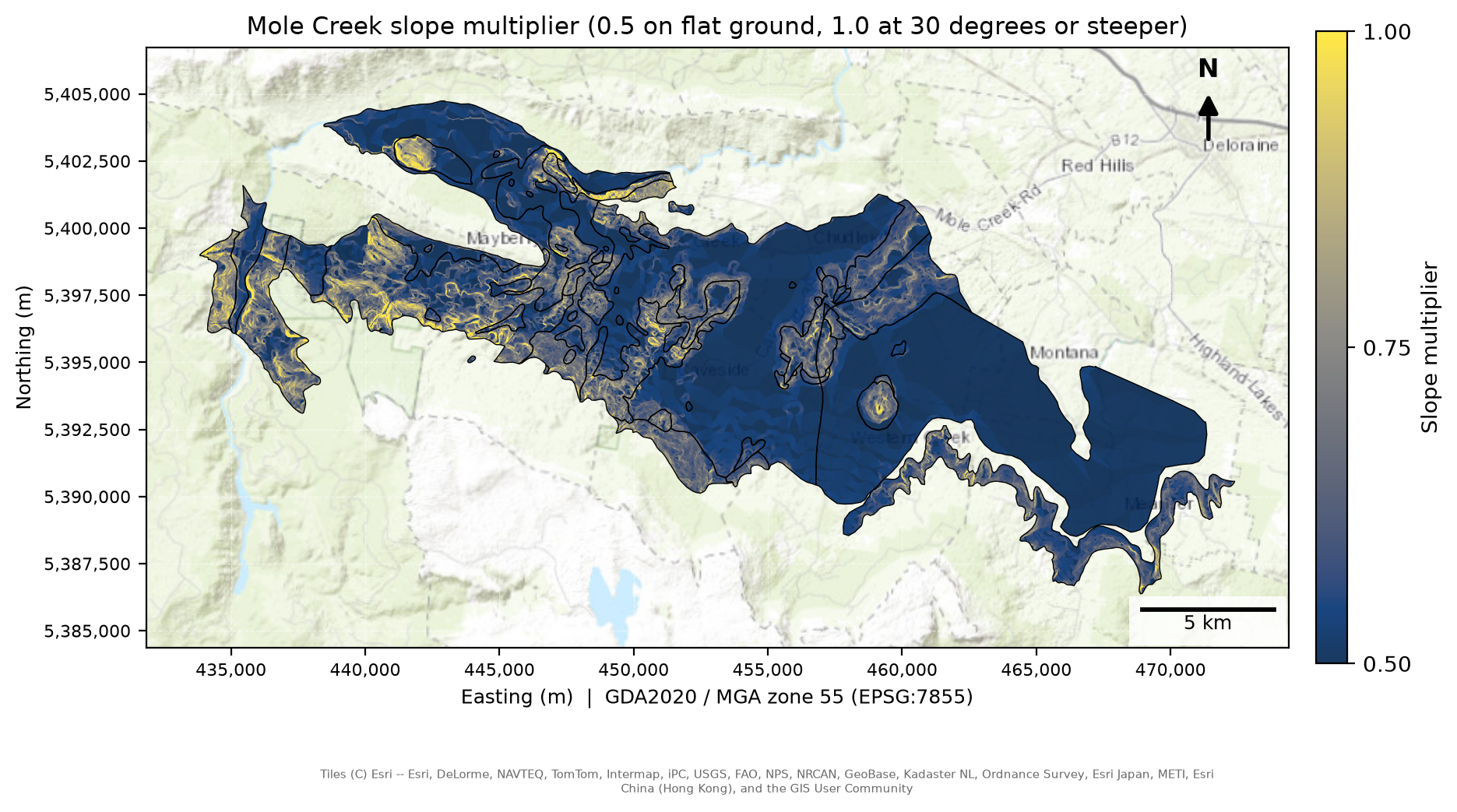
The slope multiplier on the Mole Creek karst.
Putting it together
KIVI is susceptibility × connectivity, each divided by its maximum. Multiplying by pressure and the slope multiplier gives relative risk. Risk is a product of four terms that are each below 1, so it rarely exceeds 0.5 (a strong cell scores about 0.1 with LIST pressure and exposure). It is sorted into fixed classes at 0.025, 0.05, 0.075 and 0.10: Very Low (up to 0.025), Low, Moderate, High and Very High (above 0.10), with 0 shown as None. The edges are absolute, so a label means the same score at Mole Creek and statewide, and a class stays empty if no cell reaches it.
The scores in one place
Every ingredient is scaled to 0 to 1 before it enters the equation:
| Ingredient | Raw score | Scaled by |
|---|---|---|
| Susceptibility (S) | Karst Atlas category A to D scored 4 to 1, times exposure (exposed 3, covered 2, interstratal 1), 0 for no karst | each divided by its maximum, then multiplied |
| Connectivity (C) | Four D8 log classes, scaled to 0 to 3 | divided by 3 |
| Pressure (P) | LIST land-use matrix, 0 to 10: conservation and natural land 1, plantation forestry 6, intensive uses up to 10 | divided by 10 |
| Slope | Multiplier from 0.5 (flat) to 1 (30 degrees or steeper) | used as it is |
The land-use scores are expert judgement in both versions (DEA classes in 05, the LIST matrix in src/landuse_list.py).
How the ingredients combine
Both EPIK and COP multiply their factors, while methods such as DRASTIC add weighted scores, so we run the alternatives (Stage 14):
| Structure | How the ingredients combine | Inputs |
|---|---|---|
| Product (main) | S × C × P × slope | The four ingredients above |
| Same inputs, all summed | A weighted sum of S, C, P and slope, zero off the karst; equal weights and 3:3:2:1 | The same four |
| Six-input weighted sum | Equal weights over susceptibility, exposure, catchment flags, watercourse, slope and rainfall, then × P | Six inputs, closer to a literature-style index |
| EPIK and COP replications | EPIK’s 3:1:3:2 weights over its four analogues; COP’s O × C × P product | Each method’s own factors |
Keeping the inputs the same in the first two rows separates the effect of structure from the effect of data.
The main product (left) against the four ingredients added with equal weights (right), Mole Creek. The two are on different scales (the sum scores 0.4 to 0.5, the product mostly under 0.1), so each map is split into fifths of its own karst cells: the colours show where each map ranks a cell.
How slope enters
Slope is part of the method too. Published rules differ, and COP (Vías et al., 2006) gives slope two signs, so we run our rule against COP’s and against lower ceilings (Stage 9, section 9.7):
| Rule | Direction | Form |
|---|---|---|
| Ours (main) | Steeper = higher | Continuous, 0.5 to 1 at 30 degrees |
| Lower ceilings | Steeper = higher | Continuous, reaching 1 at 20, 15 or 10 degrees |
| COP Scenario 1 (water draining to a swallow hole) | Steeper = higher | Four classes at 8%, 31% and 76% slope (4.6, 17.2 and 37.2 degrees) |
| COP Scenario 2 (diffuse recharge on the karst itself) | Flatter = higher, because runoff on steep ground leaves the karst | The same four classes, reversed |
COP’s vegetation split is dropped because pressure already scores land cover.
Conservation priority
The Conservation of Freshwater Ecosystem Values (CFEV) Integrated Conservation Value (ICV) layer rates karst as Moderate, High or Very High. We rasterise it onto the 100 m KIVI grid, give each cell the class that covers most of its area, and keep the cells that have both a KIVI score and an ICV class. KIVI is grouped into Lower (up to 0.1875), Middle (0.25 to 0.375) and Higher (0.5 and above), and each group is combined with the ICV classes to make a conservation-vulnerability priority matrix. These 9 cells are allocated into four conservation priority classes (Stage 7b, Results section 7). The group boundaries are provisional.
Conservation-vulnerability priority matrix
| Intrinsic vulnerability | CFEV Moderate | CFEV High | CFEV Very High |
|---|---|---|---|
| Higher (0.5–1.0) | Priority 3 — Moderate | Priority 2 — High | Priority 1 — Highest |
| Middle (0.25–0.375) | Priority 3 — Moderate | Priority 3 — Moderate | Priority 2 — High |
| Lower (0.041667–0.1875) | Priority 4 — Lower | Priority 4 — Lower | Priority 3 — Moderate |
Interactive map
The interactive map (Stage 15) shows the 100 m statewide results as two layers. Relative risk is coloured by each cell’s rank among the karst cells, and KIVI uses five blue classes, the same as the static maps. Clicking a karst system gives its category, exposure, connectivity class, mean slope and mean risk.
Scaling up to Tasmania
The same code (src/karst.py, src/landuse.py, src/hydro.py) runs statewide at 100 m, with the same fixed classes, the same connectivity breaks and the same 0 to 1 scale. To see what the coarser grid costs, we resample the statewide result onto the Mole Creek grid (nearest neighbour) and compare the two surfaces over the Mole Creek karst. Stage 8 compares risk and Stage 8b compares KIVI.
How we tested it
Scale. Does the 100 m statewide run reproduce the 25 m local pattern, and does routing on a 2 m DEM change the Mole Creek map?
Data. Does swapping LIST land use for DEA land cover change the map? We also rerun the model on each DEA year from 1988 to 2024 and compare the years with each other (Stage 9).
Method. Does adding weighted scores instead of multiplying them, or a different slope rule, change the map, and does it change how well springs line up with the scores?
Independent data. Do mapped springs line up with the scores? Each spring takes the score of its nearest karst polygon, and the average for the systems holding springs is compared with random draws of karst. The springs data is never an input to the model.
Sensitivity
The three tests above vary the choices the Introduction names. The model also rests on smaller judgement calls, and each is run once against the main map (Stage 9):
| Judgement | Main choice | What we varied |
|---|---|---|
| Catchment averaging of pressure | Mean over each named system, polygons within 1 km chained | No averaging; other distance thresholds |
| Weights | Equal (each ingredient to the power 1) | Each ingredient doubled in turn |
| Pressure scores | LIST matrix, 0 to 10 | For the DEA version: natural land at 0; a milder 1:2 contrast |
| Rainfall | Not used | A 0.5 to 1 modifier from the Atlas rainfall field |
Every test, and these judgement calls, is scored on one measure in Stage 16: the rank correlation with the main map over the mapped karst. The land-cover year is a change to track over time, and the final map uses 2021 land use.
Reproducibility
The pipeline is 19 stages, run in numbered order, sharing code in src/
(05b builds the LIST pressure layer that Stage 6 uses, and 05 is the DEA alternative). Three further routing runs compute the D8
flow routing that feeds the connectivity score: 03alt3 (25 m DEM) for
Mole Creek, 03-100m-hydrological-connectivity (100 m DEM) for all of
Tasmania, and 03alt2 (2 m DEM, Mole Creek) for the scale check. They sit
before Stages 3 and 7 and are not part of the numbered run: the routing is
slow and the 2 m run is too large to repeat, so their count tables are shared
outputs that Stages 3, 7 and 13 read. Raw data and those tables stay in a
shared folder, every other output is regenerated by the stages, and
environment.yml pins the conda environment.
The steps, in order:
Study areas and setup (00–01)
Susceptibility, connectivity and intrinsic vulnerability (02–04, with exposure in
04_v2)Land-use pressure, DEA (05) and LIST (05b), and relative risk (06)
Statewide run, conservation value and scale comparison (07, 07b, 08 and 08b)
Sensitivity and validation (09, 10)
Connectivity across resolution, springs test and the Atlas check (13)
The method test: product against weighted sum, with EPIK and COP replications (14)
The interactive risk map on the Results page (15)
Which choices move the map: one comparison of every test on a single measure (16)